Partial Fraction Decomposition 

Partial-fraction decomposition is the process of starting with the simplified answer and taking it back apart, of "decomposing" the final expression into its initial polynomial fractions. To decompose a fraction, you first factor the denominator. Let's work backwards from the example above. The denominator is x2 + x, which factors as x(x + 1). Then you write the fractions with one of the factors for each of the denominators. Of course, you don't know what the numerators are yet, so you assign variables (usually capital letters) for these unknown values: A/x + B/(x + 1) Then you set this sum equal to the simplified result: (3x + 2)/[x(x + 1)] = A/x + B/(x + 1) Multiply through by the common denominator of x(x + 1) gets rid of all of the denominators: multiply each term by [x(x + 1)] / 1 3x + 2 = A(x + 1) + B(x)

Sequence and Series

A "sequence" (or "progression", in British English) is an ordered list of numbers; the numbers in this ordered list are called "elements" or "terms". A "series" is the value you get when you add up all the terms of a sequence; this value is called the "sum". For instance, "1, 2, 3, 4" is a sequence, with terms "1", "2", "3", and "4"; the corresponding series is the sum "1 + 2 + 3 + 4", and the value of the series is 10. A sequence may be named or referred to as "A" or "An". The terms of a sequence are usually named something like "ai" or "an", with the subscripted letter "i" or "n" being the "index" or counter. So the second term of a sequnce might be named "a2" (pronounced "ay-sub-two"), and "a12" would designate the twelfth term. Note: Sometimes sequences start with an index of n = 0, so the first term is actually a0. Then the second term would be a1. The first listed term in such a case would be called the "zero-eth" term. This method of numbering the terms is used, for example, in Javascript arrays. Don't assume that every sequence and series will start with an index of n = 1.

Graphing Systems of Inequalities

Once you've learned how to graph linear inequalities, you can move on to solving systems of linear inequalities. A "system" of linear inequalities is a set of linear inequalities that you deal with all at once. Usually you start off with two or three linear inequalities. The technique for solving these systems is fairly simple. Here's an example. Solve the following system: 2x – 3y < 12 x + 5y < 20 x > 0 Just as with solving single linear inequalities, it is usually best to solve as many of the inequalities as possible for "y" on one side. Solving the first two inequalities, I get the rearranged system: y > ( 2/3 )x – 4 y < ( – 1/5 )x + 4 x > 0

"Solving" systems of linear inequalities means "graphing each individual inequality, and then finding the overlaps of the various solutions". So I graph each inequality, and then find the overlapping portions of the solution regions.

Cramer's Rule

Given a system of linear equations, Cramer's Rule is a handy way to solve for just one of the variables without having to solve the whole system of equations. They don't usually teach Cramer's Rule this way, but this is supposed to be the point of the Rule: instead of solving the entire system of equations, you can use Cramer's to solve for just one single variable. 

Let's use the following system of equations: 

2x + y + z = 3 

x – y – z = 0 

x + 2y + z = 0

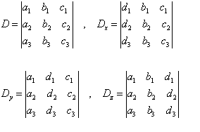
We have the left-hand side of the system with the variables (the "coefficient matrix") and the right-hand side with the answer values. Let D be the determinant of the coefficient matrix of the above system, and let Dx be the determinant formed by replacing the x-column values with the answer-column values:

Systems of Equations 

A system of equations is a set or collection of equations that you deal with all together at once. Linear equations (ones that graph as straight lines) are simpler than non-linear equations, and the simplest linear system is one with two equations and two variables. Think back to linear equations. For instance, consider the linear equation y = 3x – 5. A "solution" to this equation was any x, y-point that "worked" in the equation. 

So (2, 1) was a solution because, plugging in 2 for x: 

3x – 5 = 3(2) – 5 = 6 – 5 = 1 = y 

On the other hand, (1, 2) was not a solution, because, plugging in 1 for x: 

 3x – 5 = 3(1) – 5 = 3 – 5 = –2

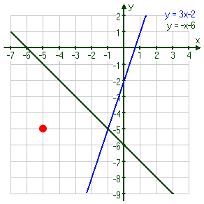
Since the two equations above are in a system, we deal with them together at the same time. In particular, we can graph them together on the same axis system.

A solution for a single equation is any point that lies on the line for that equation. A solution for a system of equations is any point that lies on each line in the system. For example, the red point at right is not a solution to the system, because it is not on either line.

Graphing Polar Equations

The most basic method of graphing polar equations is by plotting points and doing a quick sketch. Graphing polar equations is a skill that requires the ability to plot points and sometimes recognize a special case of polar curves, such as cardioids, and roses and conic sections. However, we need to understand the polar coordinate system and how to plot points for graphing polar equations. The graph of a polar equation r = f(θ), or more generally F(r, θ) = 0, consists of all points P that have at least one polar representation (r, θ) whose coordinates satisfy the equation. EXAMPLE: Sketch the polar curve θ = 1. Solution: This curve consists of all points (r, θ) such that the polar angle θ is 1 radian. It is the straight line that passes through O and makes an angle of 1 radian with the polar axis. Notice that the points (r, 1) on the line with r > 0 are in the first quadrant, whereas those with r < 0 are in the third quadrant.
And these are the polar equations that I had created.

Polar Coordinates

The polar coordinates r (the radial coordinate) and theta (the angular coordinate, often called the polar angle) are defined in terms of Cartesian coordinates by:

 x = rcostheta (1) y = rsintheta

where r is the radial distance from the origin, and theta is the counterclockwise angle from the x-axis. In terms of √(x^2+y^2) (3) theta = tan^(-1)(y/x). (4) (Here, tan^(-1)(y/x) should be interpreted as the two-argument inverse tangent which takes the signs of x and y into account to determine in which quadrant theta lies.) It follows immediately that polar coordinates aren't inherently unique; in particular, (r,theta+2npi) will be precisely the same polar point as (r,theta) for any integer n. What's more, one often allows negative values of r under the assumption that (-r,theta) is plotted identically to (r,theta+/-pi).

We start with a cartesian coordinate system. We choose O as pole and the x-axis as polar-axis. The cartesian coordinates of a point P are (x,y). Choose the u-axis such that r > 0. then P = r U => P2 = r2 U2 => x2 + y2 = r2 r = sqrt(x2 + y2) Now, choose a t-value such that x = r.cos t and y = r.sin t